
Understanding the balance of risk and return is fundamental to making informed investment decisions.
To do this, key risk statistics are needed to quantify and compare investments across a suite of different investment types. By dissecting these metrics through formulas, examples, and practical interpretations, we aim to provide a clear framework for evaluating investments.
Whether you're evaluating a single stock, a tactical strategy, or a blend of strategies, different risk measures should be prioritized based on the type of investment.
This blog is meant to serve as a guide to understanding risk statistics.
Contents:
Alpha
Batting Average
Beta
Correlation
Maximum Drawdown
Sharpe Ratio
Sortino Ratio
Standard Deviation
Tracking Error
Ulcer Performance Index
Up/Down Capture
Alpha
Alpha is a statistical measure that compares an investment to a benchmark. It is the excess return generated after accounting for beta to the benchmark.
As Morningstar puts it, "A positive alpha indicates the investment has performed better than its beta would predict. A negative alpha indicates an investment has underperformed, given the investment's beta."
Alpha Components
Investment Return: for longer periods this is generally annual return and for shorter periods this is total return. The key is that this, and the return of the benchmark, are consistent.
Risk-Free Rate: a short-term U.S. government debt obligation.
Beta: a measure of how much an investment moves relative to a benchmark.
Benchmark Return: This is the same calculation as component one, applied to the benchmark.
Step by Step Calculation
Step one is to subtract the risk-free rate from the return of the investment. This shows the excess return generated above what could have been achieved with little or no risk:
Investment Return - Risk-Free Rate
Step two is to subtract the risk-free rate from the benchmark return. Again, this shows the excess return generated by the benchmark above what could have been achieved with little or no risk.
Benchmark Return - Risk-Free Rate
Step three is to calculate the investment's expected return. This is done by multiplying the investment's beta by the number calculated in step 2 (Benchmark excess return).
Beta x (Benchmark Return - Risk-Free Rate)
The last step is to subtract the result of step three from the result of step one above.
This is alpha - the return of the investment above what is expected.
Application
Alpha is what all active strategies seek. An alpha above zero shows that an investment or strategy has outperformed its benchmark after adjusting for beta (see below). An alpha below zero shows the opposite, that the investment didn't outperform the benchmark after adjusting for beta.
For example:
Investment Return = 10%
Risk-Free Rate = 3%
Beta of the investment = 1.1
Benchmark Return = 8%
Alpha = ( 10% - 3% ) - 1.1 x ( 8% - 3% ) = 1.5%
So, the investment had an alpha of 1.5%. The return was 1.5% greater than expected based on beta to the benchmark.
Potomac's Perspective
Alpha measures an investment's return above its expected return. The expected return is calculated by multiplying the investment's beta by the benchmark excess return.
A positive Alpha indicates skill or added value, while a negative Alpha suggests underperformance on a risk-adjusted basis.
Alpha is a key metric for evaluating performance relative to a benchmark but should be used alongside other tools and considered in context.
Batting Average
In investing, batting average is a metric used to evaluate how often a fund or strategy outperforms its benchmark over a defined period. It measures consistency of outperformance, not magnitude, and answers the question: "What percent of the time did this strategy beat the benchmark?"
Batting average considers whether you got a hit (therefore beating the pitcher/benchmark) without concern or measurement of whether the hit was a single, double, or home run. It is simply: "How many times did you beat the benchmark during the period reviewed?".
This is why It is critical to combine batting average with other metrics in this document such as up/down capture or Sortino Ratio.
Why Use Batting Average?
Most performance metrics evaluate only risk and return. What they don't account for is how consistently a manager beats the benchmark.
Two managers could have the same overall return, but one may outperform in more months (more consistent), while the other may outperform in fewer but more significant months.
Formula
Batting Average = Number of outperforming periods / total periods
Periods are equal to the timeframe chosen and are most commonly months or years.
Step-by-Step Calculation
Define the Time Frame
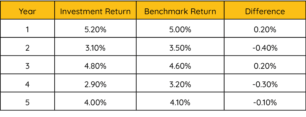
Choose a consistent period to evaluate performance. In the example, we will calculate a 5-year batting average.
Compare Returns for Each Period
Look at whether the investment outperformed the benchmark in each year.
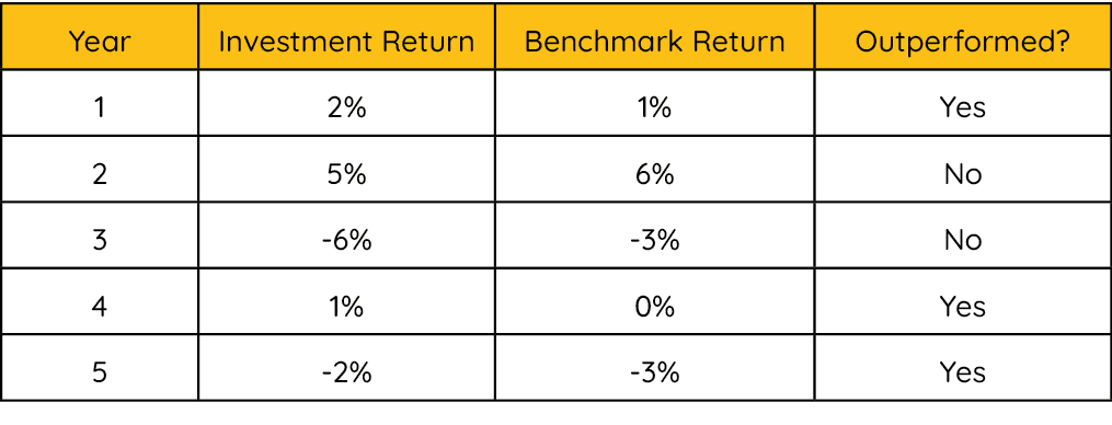
Divide the outperforming years by total years.
The investment outperformed the benchmark in three of the five years.
3/5 = 60%
In this case, the batting average is 60% and represents the percentage of time the investment outperformed its benchmark.
Interpreting Batting Average
100%: The strategy beat the benchmark in every period.
50%: The strategy beat the benchmark exactly half the time.
Below 50%: Underperformed more than half of the time.
Above 50%: Outperformed more than half of the time.
Potomac's Perspective
Batting average measures how often a strategy outperforms its benchmark-not by how much.
A higher batting average indicates greater consistency in outperformance.
It should be used in combination with other performance metrics to get a complete picture of risk-adjusted returns.
This is an important point for tactical strategies like ours. We may have a lower batting average due to risk management, but over time the months/years that we outperform can be the most important ones.
To put it simply, outperforming when the market has a major drawdown is more significant than slight underperformance during a bull market
Beta
Beta is a measure of an investment's sensitivity to overall market movements. It tells investors how much a security or portfolio is expected to move relative to a benchmark, typically the S&P 500.
It is a central concept in risk analysis, especially within the framework of modern portfolio theory and the Capital Asset Pricing Model (CAPM).
A beta of 1.0 means the investment moves in line with the market. A beta greater than 1.0 suggests more volatility than the market, while a beta less than 1.0 indicates less volatility.
Why Use Beta?
Traditionally, beta is used to assess the systematic risk of an investment. It provides insight into how a security is likely to behave during broad market moves.
This is important for allocators during:
Portfolio construction
Asset allocation
Measuring market risk exposure
Adjusting portfolio volatility levels
Formula
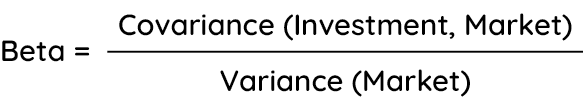
In simple terms, beta is the ratio of how much an investment moves in relation to market returns.
More precisely, it's the covariance between the investment and the benchmark divided by the variance of the benchmark.
Interpreting Beta
If the beta of a fund is 1.0, it's expected that it will move in line with its benchmark. If the beta is 2.0, the fund has historically moved twice as much as the benchmark.
So, if the benchmark is up 2%, we'd expect a fund with a 2.0 beta to be up 4%. If the benchmark is down 2%, we'd expect the fund to be down 4%.
Beta quantifies the volatility of a fund compared to a benchmark.
Potomac's Perspective
Beta is a foundational metric in risk analysis that measures how sensitive an investment is to movements in the broader market.
However, it doesn't tell the full story. For strategies that aren't fully invested at all times, beta can be misleading.
A tactical strategy that can go from cash to an exposure greater than 1.0 beta might have an overall beta, measured over a longer cycle, that doesn't accurately describe the day-to-day experience.
It's important to realize that beta is a long-term measure designed for fully invested funds or strategies. Anything that deviates from that requires deeper understanding to gain the full context of beta.
Correlation
Correlation is a statistical measure that expresses the strength and direction of a relationship between two variables. In investing, it tells us how closely the returns of two assets move in relation to one another.
Correlation values range from -1 to +1:
+1: Perfect positive correlation - the assets move exactly in the same direction.
-1: Perfect negative correlation - the assets move in exactly opposite directions.
0: No correlation - the movements are unrelated.
Why use Correlation?
The degree to which two investments move in relation to one another can have a significant impact to the overall portfolio.
If two assets have positive long-term returns and one asset always declines while the other rises, the overall portfolio volatility is reduced and true diversification is achieved.
Allocators aim to include investments which have low correlation to each other in order to reduce volatility and maximum drawdown.
Formula
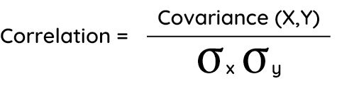
Where:
X and Y are the return series of the two investments
σ represents standard deviation
Interpretation
The Oxford Dictionary defines correlation as "a mutual relationship or connection between two or more things."
More specifically, it measures the degree of co-movement between variables using a bounded indicator that falls between +1 and -1. In the extremes, correlation is either +1 or -1, where the variables move perfectly in unison or exactly inverse to each other.
To illustrate, imagine two vehicles traveling on a highway. They can travel in the same direction, in opposite directions, or without relativity at all.
Correlation operates in this way. It does not account for the speed of the cars, only direction.
There are three possible states: positive, negative, and zero with a range of -1 to 1.
Potomac's Perspective
Correlation is a critical piece of the asset allocation puzzle. It is a quantifiable way to see if one investment is different from another.
The word tactical is one of the most abused naming conventions in our industry. Just because you add the word "tactical" to the name of the strategy doesn't mean much because of the various definitions of the word. We feel that correlation is one of the statistics to uncover whether a strategy is truly tactical or not.
If the broad equity market, as measured by the S&P 500 (correlation of 1), is the benchmark, the long-run correlation of an investment strategy should be below 0.70 to provide a truly differentiated experience.
The real-life experience is that most tactical is "in name only." Many tactical investments aren't truly tactical. Their correlations are above 0.80 and, therefore, don't provide much of a diversification benefit to the overall portfolio.
Maximum Drawdown
Maximum drawdown is a risk metric that measures the largest peak-to-trough decline in the value of an investment or portfolio during its trading history. It helps investors understand the worst-case loss scenario in terms of percentage decline.
Rather than focusing on day-to-day volatility, the maximum drawdown is a snapshot that reflects the pain of holding an investment - the worst loss an investor would have experienced by owning it.
Why Use Maximum Drawdown?
Investors often focus on returns and overlook the fact that they may not have been able to endure the losses along the way. By quantifying the worst loss, drawdown gives insight into what the experience could be going forward.
Drawdown also allows for an apples-to-apples comparison between investments. This is useful to see how different investment options manage risk during major declines.
Formula
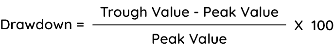
Maximum Drawdown is always expressed as a negative percentage, representing the maximum percentage loss from a prior peak.
Step-by-Step Calculation
1. Identify the Peak
Record the historical value of the highest point (peak value) before a decline.
2. Find the Trough
Record the lowest point (trough value) that follows the peak.
3. Apply the Formula
If an investment peaked at $100 and dropped to $65 (trough):
Maximum drawdown = ( $65 - $100 ) / $100 * 100 = -35%
This indicates a 35% maximum drawdown-the worst decline the investment experienced during the period.
Potomac's Perspective
At Potomac, alpha, beta, and other metrics provide some value, but the historical maximum loss is a critical risk measure and is given priority. Why? Because maximum drawdown is "the ride you take."
Here are three points to summarize our view on why maximum drawdown is one of the most important metrics:
There has been extensive work done which shows that investors treat losses differently than gains. Famed behavioral psychologists Daniel Kahneman and Amos Tversky said that "losses loom larger than gains" and found that the pain of losing is psychologically about twice as powerful as the pleasure of gaining.
The math behind frequent large losses is problematic. A 20% loss requires a 25% gain to break even. As drawdowns deepen, the math of compounding increasingly works against you. That's why we focus on minimizing drawdowns-to keep compounding working in our favor.
Annualized long-term results are often quoted, but few are actually achieved. Drawdowns are often too large and painful for investors to endure. This causes them to tap out and never realize long-term gains.
Sharpe Ratio
The Sharpe ratio is the most common performance metric for evaluating risk-adjusted returns. It calculates the excess return of an investment relative to its risk, as measured by the standard deviation.
In layman's terms, "how much did you earn above the safest investment based on the risk you took to earn it?"
Components of the Sharpe Ratio
Average Annual Return - How much the investment made per year, on average.
Risk-Free Rate - a short-term US government debt obligation.
Standard Deviation - a measure of volatility around average returns.
The Formula

Breaking Down the Components
Average Annual Return
Component one is as simple as it sounds. Calculate the annualized return of the investment over the time frame chosen.
For example, if using a 3-year Sharpe ratio, we annualize the returns over the last three years.
Year 1: 15%
Year 2: 5%
Year 3: 10%
The average annual return over the three-year period would be:
(15% + 5% + 10%) / 3 = 10%
Risk-Free Rate
The risk-free rate is the return of a risk-free investment, often represented by the most recent yield of a U.S. Treasury bill (T-bill). This is similar to a money market fund, which is often used in place of cash to earn a nearly risk-free yield.
For our example calculation (shown later), we will assume the 90-day Treasury Bill rate is 4.30.
Standard Deviation
Standard Deviation is how spread-out data is relative to the average. It indicates how much the returns fluctuated over a given period.
To be consistent with the example above, the three-year standard deviation is ~4%. This means that performance has typically been within 4% on either side of its average annual performance.
In the Sharpe ratio calculation, the critical point is that the standard deviation is a measure of risk and quantifies how spread-out returns have been relative to the average.
Sharpe Ratio Calculation
For the result we combine the three components into the formula shown before:
Sharpe ratio = ( average annual return - risk-free return ) / standard deviation
Sharpe ratio = ( 10% - 4.30% ) / 4% = 1.43
For this investment, the 3-year Sharpe ratio is 1.43.
Potomac's Perspective
Anyone can increase returns, in theory, by adding market risk. However, skilled managers aim for more return (or at least market returns) with less market risk.
The Sharpe ratio measures risk-adjusted performance, where risk is defined as standard deviation.
Over the long term if you are focused on "risk adjusted performance" the higher the Sharpe the better.
The most cited flaw of the Sharpe ratio focuses on its volatility component. As the formula shows, higher overall volatility results in a lower Sharpe ratio.
However, upside volatility shouldn't be penalized as no one complains about returns being too high. Sharpe places equal importance on upside and downside volatility, which is a flaw, it doesn't show favor for strategies that deliver more upside than downside.
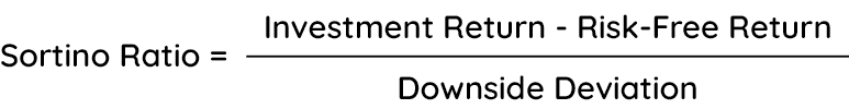
Sortino Ratio
The Sortino Ratio is a performance metric used to evaluate an investment's risk-adjusted return, similar to the Sharpe ratio, but with a key difference-it only considers downside volatility.
By focusing exclusively on standard deviation of negative returns, the Sortino Ratio provides a more precise measure for investors who are primarily concerned with downside risk.
Why Use the Sortino Ratio?
Traditional risk measures, such as standard deviation, treat upside and downside volatility equally. However, investors typically welcome upside volatility (large up moves) and are only concerned with downside risk.
The Sortino Ratio corrects this flaw by only considering volatility from negative returns, making it a more realistic metric for evaluating risk-adjusted performance.
Formula
Breaking Down the Components
Average Annual Return
Calculate the annualized return of the investment over the time frame chosen.
For example, if we want a 3-year Sortino ratio, annualize the returns over the last three years.
Year 1: 15%
Year 2: 5%
Year 3: 10%
The average annual return over the three-year period would be:
(15% + 5% + 10%) / 3 = 10%
Risk-Free Rate
The risk-free rate is the return of a risk-free investment, often represented by the most recent yield of a U.S. Treasury bill (T-bill). This is similar to a money market fund, which is often used in place of cash to earn a nearly risk-free yield.
For our example calculation (shown later), we will assume the current 4-week Treasury Bill rate is 4.27%.
Downside Deviation
This is the standard deviation for months where returns were negative. For instance, if month one had a return of +5%, month two had -2%, and month three had +3%, we would compute the standard deviation solely based on month two, as it had a negative return.
Sortino Ratio Example
Suppose an investment has the following characteristics:
Annualized Return: 10%
Risk-Free Rate: 4.27%
Downside Deviation: 5%
Using the formula:
(10% - 4.27%) / 5% = 1.15
The investment has a Sortino Ratio of 1.15, meaning that it earned 1.15 units of excess return per unit of downside risk.
Potomac's Perspective
Are you really going to penalize a manager for delivering "upside vol?"
The Sortino Ratio improves upon the Sharpe Ratio by considering only downside risk.
A higher Sortino Ratio suggests that an investment has generated strong returns with minimal relative downside volatility. This is an improvement over the Sharpe ratio as investors typically don't mind their returns being volatile on the upside.
Standard Deviation
Standard deviation is a key statistical measure used to assess the volatility or risk of an investment by showing how much its returns vary from the average. It's widely used to understand the consistency of an investment's performance over time.
It answers the question: "How much do returns typically vary around the average?" A higher standard deviation signals greater volatility, while a lower one suggests stability.
Breaking Down the Formula
Before looking at the different components of the formula, note that standard deviation is a complex measure to calculate. Memorizing the steps of calculation isn't necessary or particularly useful day to day, though knowing the general process gives insight into what the end number represents.
Average Return
First, you must calculate the average return over a chosen period. This is the baseline that standard deviation measures against. Usually, this is the average annual return. Let's assume that an investment has the following returns over the past three years:
Year 1: 12%
Year 2: 4%
Year 3: 8%
The average return is simply: (12% + 4% + 8%) / 3 = 8%
Deviations from the Average
Next, calculate how much each year's return deviated from the average:
Year 1: 12% - 8% = 4%
Year 2: 4% - 8% = -4%
Year 3: 8% - 8% = 0%
Variance
The last step before we calculate the final number is to square these deviations (to remove negatives), then average them:
Year 1: (4%)² = 16%
Year 2: (-4%)² = 16%
Year 3: (0%)² = 0%
Variance = (16% + 16% + 0%) / 3 = 10.67%
Finally - Standard Deviation
Take the square root of the variance to get standard deviation: √10.67% ≈ 3.27%
So, this investment's standard deviation is roughly 3.27%.
Interpretation and Use Case - How to Use Standard Deviation
Most often, standard deviation is used to measure volatility of an investment relative to another. For example, if fund A has a 5% standard deviation and fund B has one of 10%, then we could say that fund B has a volatility that is double that of fund A.
The second method of interpretation focuses only on a single investment. Mathematically, this means that:
68% of the time, returns stay within one standard deviation.
95% of the time, returns stay within two standard deviations.
99% of the time, returns stay within three standard deviations.
For those who remember taking an introductory statistics class, these metrics should be easily recognizable as the normal distribution...or the bell curve.
Let's say that the investment has a 5% standard deviation and an average annual return of 10%. This means that the annual return has fluctuated in a range of 5% to 15% (10% ± 5%) 68% of the time.
Standard Deviation: 68% of the time the investment's annual return has been between 5% and 15%. This represents one standard deviation above and below the average return.
Standard Deviations: The math indicates that 95% of the time, returns will fall between 0% and 20% (10% ± 10%).
Standard Deviations: Readings beyond three standard deviations can be considered outliers. Unlike in statistics, however, in markets outliers happen more often than the normal distribution would have you believe. Markets have "fat tails."
To put it simply, standard deviation is a number that represents the volatility around the average return of the investment. 68% of the time an investment has stayed within one standard deviation of the average and 95% of the time it has stayed within two.
An investment with a higher standard deviation can be expected to deviate from its average return more than an investment with a lower standard deviation.
Likewise, an investment with a high standard deviation is less likely to deliver the "average" return in a given year.
Comparing two investments by their standard deviation provides a snapshot of each fund's volatility and determines which is more volatile.
Potomac's Perspective
Standard deviation measures how spread out an investment's returns are around its average, making it a go-to metric for gauging risk.
A higher value indicates more volatility, which might mean bigger gains but also bigger losses. A lower value points to steadier performance because there is less variation around its average return.
While it's a cornerstone of risk analysis, it treats upside and downside deviations equally, so it should be paired with other tools, such as the Sortino Ratio, for a fuller picture.
Tracking Error
Tracking error is a performance metric that measures how closely an investment follows the returns of its benchmark index. It quantifies the degree to which an investment's return deviates from the benchmark, helping investors evaluate performance relative to another investment.
A lower tracking error indicates that the investment is closely aligned with the benchmark, while a higher tracking error suggests greater deviations.
Tracking error, in itself, is not a measure of success or failure. A high tracking error may not necessarily be a bad thing - if you want to differ from your benchmark, you must do something different from your benchmark. This is why tracking error should be taken with context on what the investment's objective is.
Side Note
As with standard deviation, memorizing the steps of calculation isn't necessary or particularly useful day to day. However, understanding the general process gives insight into what the final number represents.
Breaking Down the Formula
Tracking error is calculated as the standard deviation of the difference between the investment's returns and the benchmark's returns over a specified period.
So, for a 5-year tracking error, the final number represents the average annual deviation of the investment's performance relative to the benchmark over those five years.
Formula:
Tracking Error = Standard Deviation of (Investment return - Benchmark return)
Step-by-Step Calculation:
Step 1: Calculate Return Differences
First, determine the difference between the investment return and the benchmark return for each period.
For example, consider the following returns over a 5-year period:
Step 2: Take the Standard Deviation of the Differences
For the steps on how to calculate standard deviation, refer to the standard deviation section.
As you will read, standard deviation isn't a simple measure and that section must be read to fully understand it.
By taking the standard deviation of the differences, our tracking error from the five-year period is 0.25%.
Interpreting Tracking Error
Now that the tracking error has been calculated, it must be interpreted.
Using the same number as before, the five-year tracking error is 0.25%. This means that over this period the average deviation of the investment from its benchmark was 0.25% per year.
It's important to take each tracking error in the context of the type of fund. Passive index funds should track the index closely, and anything above 1% would be considered negative.
Potomac's Perspective
For tactical strategies that aim to look different than any benchmark, tracking error may be high. We would argue that a tactical manager with low tracking error is not really a true tactical manager.
When this is the strategy's objective - to be independent of any index - benchmark selection becomes difficult.
Deviations from the benchmark can be a good thing - especially if they are due to differing performance during a market decline. In this scenario, tracking error will be high and should be interpreted as a benefit.
Ulcer Performance Index
Ulcer Performance Index (UPI)
The Ulcer Performance Index (UPI) is a risk-adjusted return metric that penalizes drawdowns - both depth and duration.
This makes UPI particularly useful for strategies that emphasize risk reduction and minimizing drawdowns. It is one of the few metrics that gives insight into risk adjusted returns through the lens of drawdown.
Why Use UPI?
Traditional performance metrics often fall short in capturing the psychological pain investors experience during extended downturns. The Ulcer Performance Index was created to reflect how uncomfortable the ride was.
UPI helps investors evaluate how severe declines were and how long they lasted.
Formula
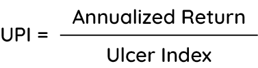
Where the Ulcer Index is a measure of drawdown severity over time. Technically it is the root mean square from peak values over the period. In plain terms, it is a method to penalize drawdown severity and duration.
Step by Step Calculation
Calculate Drawdowns Over a Selected Period
For each period, calculate the percentage decline from the most recent peak.
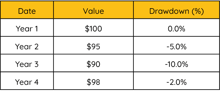
Square the Drawdowns, average them, and take the square root. This gives us the Ulcer Index.
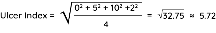
Divide the Annualized Strategy Return by the Ulcer Index
If the strategy had an annualized return of 10.0%, the UPI would be:
10% / 5.72 = 1.75
Interpreting UPI
As with other ratio-based measures, anything above 1.0 means the investment's return compensated the investor for the risk they experienced. For UPI, a ratio above 1.0 means the returns compensated the investors for the drawdown severity they endured. In this case, severity is taken to mean depth and duration of drawdowns.
The second way UPI can be used is to measure two investments against each other. It can be a good way to determine which are the riskiest in terms of drawdown adjusted returns.
Some simple things to keep in mind for UPI:
Higher is better. A higher UPI means the strategy delivered more return per unit of downside risk.
Unlike the Sharpe or Sortino ratios, UPI gives you an idea of how comfortable it was to stay invested through the lense of drawdown.
A UPI above 1.0 is generally seen as favorable.
Potomac's Perspective
Not all drawdowns are created equally, even when they are equal. Take two investments, A and B. Both have a drawdown of 30%. However, the drawdown for investment A lasts twice as long as that of investment B. Which was more severe?
A 30% drawdown that quickly recovers to new highs (think COVID-era) is preferable to a similar sized drawdown that requires many years before the prior highs are regained. Human psychology generally does not allow for a person to sit in a money-losing investment for extended periods of time. Opportunity costs are real, and ulcer performance index accounts for that.
Up/Down Capture
Upside and downside capture are tools used to evaluate the performance of an investment strategy relative to a benchmark index.
These metrics help investors assess how well a strategy has performed during both positive and negative market conditions, providing insight into its relative risk and return.
Up Capture Calculation
To calculate the up-capture ratio, only consider months where the benchmark had a positive return. For those months, calculate the total compound return for both the strategy and the benchmark.
For a 10-year up-capture ratio:
Filter out months over the 10-year period where the benchmark had a negative return.
Using the remaining data, calculate the total compound return for both the strategy and the benchmark.
Divide the strategy's return by the benchmark's return.
Formula

Example:
If the benchmark's total compound return over the 10-year period was 100% and the strategy's return was 120%, the up-capture ratio would be:
120% / 100% = 120%
Remember, this is only using data for months where the benchmark was positive. So, it's the total return only during up markets.
Interpretation:
Above 100%: The investment outperformed the benchmark during rising markets.
Below 100%: The investment underperformed the benchmark during rising markets.
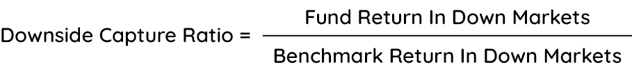
Down Capture Calculation
To calculate the down-capture ratio, the process is similar but focuses only on months where the benchmark had a negative return.
For a 10-year down capture ratio:
Filter out all months during the 10-year period where the benchmark had a positive return.
Calculate the total compound return using the remaining data.
Divide the strategy's return by the benchmark's return.
Example:
If the investment's total return in down markets over the 10-year period was -50% and the benchmark's return was -75%, the down-capture ratio would be:
-50% / -75% = 66.67%
Interpretation:
Above 100%: The investment lost more than the benchmark during down markets.
Below 100%: The investment lost less than the benchmark during down markets.
Up/Down Capture Ratio
Combining the two measures creates a powerful ratio for comparing different investment's performance relative to a benchmark. Using the same numbers as before:
Up capture: 120%
Down capture: 66.67%
When directly comparing the two, it's easy to see that this investment has had good performance relative to the benchmark. It participated in more gains than losses, outperforming in up markets while managing risk during down markets.
To create the ratio, you simply divide the up capture by the down capture:
120% / 66.67% = 1.80
In this case, the investment captured 1.80 times as much of the gains relative to losses. It outperformed in up markets, and managed risk during down markets. A ratio above 1.0 is generally a sign of strong performance.
Potomac's Perspective
Measuring the up capture and down capture ratios can provide insight into how an investment has performed against a benchmark.
An up-capture ratio greater than 100% is considered outperformance because the investment gained more in up markets than the benchmark.
A down-capture ratio less than 100% is considered outperformance, as the investment declined less than the benchmark.
Up/Down capture ratio blends the two measures to give a full view of performance. The higher the ratio, the better the relative performance and risk management.
This gives a view of how an investment performed during both market types and can highlight risk management during declines.
Conclusion
Understanding and applying these risk metrics provides investors with the tools necessary to choose the best asset combinations based on the investment type.
At Potomac, we recognize that while statistical measures like these have their place, maximum drawdown remains the most critical risk metric-the one that truly defines an investor's experience and ability to realize long-term returns.
No amount of statistical sophistication can replace the importance of knowing how much an investment has lost during adverse conditions.
By integrating these tools into your analysis, you can make more informed decisions on the tradeoff between risk and return. Whether assessing a single stock, a tactical strategy, or a diversified portfolio, different measures should be used for each.
In the end, successful investing isn't just about maximizing returns-it's about understanding and controlling the risks that come with them so that an investor is able to realize long-term total returns.


